
Period three implies CHAOS!
note on the title:this is the exact title to the 1975 paper by Yorke, an applied mathematician - who is credited with bringing back Lorenz' seminal work.Who was Lorenz?Read on!
We can relate pretty well to our intermediate school differential equations. And though they did not take as much toll as indefinite integration did - it all boiled down to some really frightening (and at times transparent) expressions that had to be moulded into a solvable form we knew of and follow the old techniques.
But we have heard of seldom-encountered-but-know-they-are-there type of UNSOLVABLE differential equations that cannot be solved. So? Some differential equations cannot be solved. We can take that in our stride right? Try this! Only some differential equations can be solved, a wider variety - infinite for all we know - are unsolvable. Its a bit like being at rest with the idea that our rational number system being infinitely dense and that makes the irrational numbers exceptions- and you get a proof out of the blue that irrational numbers are more dense on the number line, or metric space-technically speaking.
Since its inception in 1600+something , calculus has provided a novel way for studying continuous variations- infact it arose as a tool for physics (no offence to the mathematicians)- and has been the 'quantum leap' for sudy and modelling of physical systems in nature, otherwise known as PHYSICS.
An etymological observation here- quantum is a very small quantity right? so how does a 'big' leap translate to 'quantum' leap?- or is it a reference to the enormous paradigm shift the 20th century physics community had to undergo in order to accomodate the most successful theory of their time.
Returning to the main stream of thought, though the chaotic behaviour of systems (i am going to ask you to go by the 'feel' of the word here - a random unpredictable behaviour that refuses to settle down to any semblance of predictabilty) seems disorderly, it is actually deterministic-- that is you can predict, without any approximations, the outcome of some system. The science of 'Chaos'(the term was popularised by James A Yorke, an applied mathematician who is said to have rediscovered Lorenz, in his publication 'period three implies chaos') is essentially classical- there is no relativity or quantum mechanics involved here.
but people back then were being paid to find order in systems! why study disorder?But considering its simplicity and comprehensibiliy, this science started producing papers only in the late 70s and 80s becase of the stagnantic (no such word- you DO get the sense!) set of invisible rules laid down by the scientific community-> to produce a paper that was RADICAL and DYNAMIC DEPARTURE FROM ORTHODOX was suicide! To get a grant and publish papers you had to, and still have to stay away from being too original.
You have to model physical, biological or chemical systems with the existing mathematical tools- who dares to explore systems that are random and defy modelling (read predictability). Regarding the unsolvable diferential equations we were talking of, imagine a system of two or three such equations that are coupled (meaning that in a system of x,y and z, all three can appear in any form, linear or nonlinear,in each expression.) - we are trying to gauge the amount of complexity that can be built in around these systems.these system of differential equations can, however, be approximately solved using computing algorithms. so we can get a stream of data with varying time in which given a set of initial conditions mark the starting points and the system of equations mould the path of the variables. this is all the insight we need to get into the story of Edward Lorenz
"Lorenz was born in West Hartford, Connecticut. He studied mathematics at both Dartmouth College in New Hampshire and Harvard University in Cambridge, Massachusetts. During World War II, he served as a weather forecaster for the United States Army Air Corps. After his return from the war, he decided to study meteorology. Lorenz earned two degrees in the area from the Massachusetts Institute of Technology where he later was a professor for many years."--wikipedia. for all our purposes, edward lorenz was a meteorologist. during his days as weather forecaster he built a very primitive model of the climate system of earth, with a view to predict local weather. though the work was not very successful in terms of scientific design, it became famous in his department, the system of twelve interwoven differential equations churned out a stream of data on a long roll of paper (remember that this was around 1960, give or take one year on each side).people would bet on what the weather would be that day- windy, or sunny or wet. one day, so the story dictates, he wanted to start midway instead of starting allover again - putting in the same initial conditions and wait for an hour to go back where he left- instead he looked up the data in the previous sheet and fed it to the computer.this data seems to have survived for storytellers- he put in an approximation."One day in 1961, he wanted to see a particular sequence again. To save time, he started in the middle of the sequence, instead of the beginning.He entered the number off his printout and left to let it run. When hecame back an hour later, the sequence had evolved differently. Instead of the same pattern as before, it diverged from the pattern, ending upwildly different from the original. Eventually he figured out what happened. The computer stored the numbers to six decimal places in itsmemory. To save paper, he only had it print out three decimal places. In the original sequence, the number was .506127, and he had only typedthe first three digits, .506. "- http://library.thinkquest.org/3120/old_htdocs.1/text/fraz1.txt .
Although i would like to think that there was more than one variable in the calculations. this illustration does its job pretty well though, it shows that the pattern, or  sequence if you please, was very dependant on the initial conditions. For practical purposes, an experimentalist prides himself if he can determine a physical quantity to the third decimal place. Here the absence of the fourth, fifth, and sixth decimals had erased all similarities to the original sequences within three-four cycles. What lorenz aptly demonstrated after this was that long term weather prediction was impossible. To do so he stripped down his system of equations for convection to their bare essence to three eqations.afterwards it was discovered that his equations mimicked a water-wheel- "At the top, water drips steadily into containers hanging on the wheel's rim. Each container drips steadily from a small hole. If the stream of water is slow, the top containers never fill fast enough to overcome friction, but if the stream is faster, the weight starts to turn the wheel. The rotation might become continuous. Or if the stream is so fast that the heavy containers swing all the way around the bottom and up the other side, the wheel might then slow, stop, and reverse its rotation, turning first one way and then the other. " (James Gleick, Chaos - Making A New Science, pg. 29).This is a system of equations of the same family, or perhaps the same set that lorenz used, you can try plotting the behaviour of this system at home.
 sequence if you please, was very dependant on the initial conditions. For practical purposes, an experimentalist prides himself if he can determine a physical quantity to the third decimal place. Here the absence of the fourth, fifth, and sixth decimals had erased all similarities to the original sequences within three-four cycles. What lorenz aptly demonstrated after this was that long term weather prediction was impossible. To do so he stripped down his system of equations for convection to their bare essence to three eqations.afterwards it was discovered that his equations mimicked a water-wheel- "At the top, water drips steadily into containers hanging on the wheel's rim. Each container drips steadily from a small hole. If the stream of water is slow, the top containers never fill fast enough to overcome friction, but if the stream is faster, the weight starts to turn the wheel. The rotation might become continuous. Or if the stream is so fast that the heavy containers swing all the way around the bottom and up the other side, the wheel might then slow, stop, and reverse its rotation, turning first one way and then the other. " (James Gleick, Chaos - Making A New Science, pg. 29).This is a system of equations of the same family, or perhaps the same set that lorenz used, you can try plotting the behaviour of this system at home.
(i)Dx=10*(y-x)
(ii)Dy=-x*z+28*x-y
(iii)Dz=x*y-(8/3)*z
for starters, D=> d/dt(operator);x*y='x' multiplied by 'y'
Whenever physicists encounter such a system they try to think of a quantity that is conserved, or in special cases, show predictable behaviour. Think of the simple harmonic equation D**2(x)=-w*x['**'=>raised to the power; here D**2=>d/dt(d/dt)]. in "phase space"- in which all possible states of the system is representable- this translates into a circle.Please note that lorenz was not aware of this terminology because this field of mathematics came in 1971. Say for turbulent flow in a cylindrical pipe, the elements of water that collide with the cylindrical wall, act as if it is attracted by the centre of the cross section of the pipe- THAT, thus, is the attractor in this system.Note that the elements that dont collide but are bound attractively to the surrounding elements also behave as if they are attracted, albiet by some different force law than inverse square. in lorenz' system, the attractor came out in the form of a double spiral.see picture.so although the momentary behaviour of the particle was seemingly random, in the long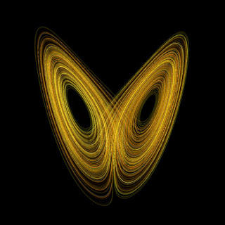 term, it was sketched out in the form of a ever-continuing, never intersecting double-spiral.sort of gives you insight into the butterfly effect- "The flapping of a single butterfly's wing today produces a tiny change in the state of the atmosphere. Over a period of time, what the atmosphere actually does diverges from what it would have done. So, in a month's time, a tornado that would have devastated the Indonesian coast doesn't happen. Or maybe one that wasn't going to happen, does. (Ian Stewart, Does God Play Dice? The Mathematics of Chaos, pg. 141)"
The bottomline in this first phase of insight into chaotic systems was that certain systems behave too sensitively to their their initial conditions and that Lorenz' work established that long-term-weather forecasting was impossible. Now comes the sadder part of it, his paper was published in a Swiss Meterological Journal that lay in obscurity waiting to be rediscovered.
The next story that defined birth of this new science was the work of Robert May, an ecologist in the 1970s. When one stands in the shoes of an ecologist and tries to model the population of, say fish in a pond, one inadvertedly realizes that the simplest model would be one in which there is unlimited food and the population of one year depends linearly on that of the previous year.i.e P(n+1)=a*P(n);P(n)=>population of the nth year.Now if you start taking into account the total food being constant,and the survival for existence, you arrive at :
Whenever physicists encounter such a system they try to think of a quantity that is conserved, or in special cases, show predictable behaviour. Think of the simple harmonic equation D**2(x)=-w*x['**'=>raised to the power; here D**2=>d/dt(d/dt)]. in "phase space"- in which all possible states of the system is representable- this translates into a circle.Please note that lorenz was not aware of this terminology because this field of mathematics came in 1971. Say for turbulent flow in a cylindrical pipe, the elements of water that collide with the cylindrical wall, act as if it is attracted by the centre of the cross section of the pipe- THAT, thus, is the attractor in this system.Note that the elements that dont collide but are bound attractively to the surrounding elements also behave as if they are attracted, albiet by some different force law than inverse square. in lorenz' system, the attractor came out in the form of a double spiral.see picture.so although the momentary behaviour of the particle was seemingly random, in the long
 term, it was sketched out in the form of a ever-continuing, never intersecting double-spiral.sort of gives you insight into the butterfly effect- "The flapping of a single butterfly's wing today produces a tiny change in the state of the atmosphere. Over a period of time, what the atmosphere actually does diverges from what it would have done. So, in a month's time, a tornado that would have devastated the Indonesian coast doesn't happen. Or maybe one that wasn't going to happen, does. (Ian Stewart, Does God Play Dice? The Mathematics of Chaos, pg. 141)"
The bottomline in this first phase of insight into chaotic systems was that certain systems behave too sensitively to their their initial conditions and that Lorenz' work established that long-term-weather forecasting was impossible. Now comes the sadder part of it, his paper was published in a Swiss Meterological Journal that lay in obscurity
 waiting to be rediscovered.
The next story that defined birth of this new science was the work of Robert May, an ecologist in the 1970s. When one stands in the shoes of an ecologist and tries to model the population of, say fish in a pond, one inadvertedly realizes that the simplest model would be one in which there is unlimited food and the population of one year depends linearly on that of the previous year.i.e P(n+1)=a*P(n);P(n)=>population of the nth year.Now if you start taking into account the total food being constant,and the survival for existence, you arrive at :
P(n+1)=a*P(n)*[b-P(n)]
If we want to capture the essence of the equation in , x(next)=r*x(present)*[1-x(present)]- this is the logistic difference equation that can be used to model a biological system in a closed ecological system.Believe me when i say that this is only an approximation, and is probably arrived on by hit and trial rather than some deep insight into the factors of demography. Certainly, this is an accepted recurrence relation only because it yields the results, i.e. it can mimic, within permissible errors, the population of certain ecological systems like that of fish in a pond,instead of being the the factor for the population variation. The least we can do to explore this field of the logistic equation is to study the patterns that appear for certain values of r, or the characteristics of the demographic pattern that evolves with r:(courtesy wikipedia-'logistic map'): When r is between 0 and 1, the population heads to zero, independent of the initial population.
When r is between 1 and 2, the population quickly stabilizes on the value (r-1)/r.
When r is between 2 and 3, the population again stabilizes on (r-1)/r but oscillates around the value for a while.The rate of convergence is linear, but at r=3, the rate is excruciatingly slow - less than linear even.
With r between 3 and 3+(6)**.5[~3.45], the population oscillates between two values dependant on r.
With r between 3 and 3+(6)**.5[~3.45], the population oscillates between two values dependant on r.
With r within 3.45 and 3.54(approx), the population oscillates between 4 values forever.

With increase of r from 3.54 onwards the the population oscillates between 8 values then 16,32,64..... and on.The period of r with the same no of oscillations decreases rapidly, with the ratio between two such intervals approaching delta=4.669.... the Feigenbaum constant- whose story we shall come in with later. Now we can throw in the term period doubling cascade- think of infinitely branching arteries.
Beyond 3.57, most values exhibit chaotic behaviour, but again some values of r are there that show non-chaotic behaviour. Like 1+(8)**.5[~3.83], these are islands of stability. In fact the bifurcation map is a fractal, if you zoom in on certain areas they seem 'similar' to the whole map again.
Perhaps we got in too deep into this mathematical system than we intended to, but this isn't even starting to get technical.Robert May thus, showed how complex and beautifully simple systems like these can be at the same time.
The third story has to be that of Yorke who with Li proved that any one-dimensional system which exhibits a regular cycle of period three will also display regular cycles of every other length as well as completely chaotic orbits in 1975.Yorke's paper was named "Period three implies Chaos"- where he coined the term for use as we know it today.
For those attracted to abstract objects/theories of beauty, Smale's work on the mathematics of chaos was the first attempt that popularised the field of chaos to physics. His work can be, at its very basic simplification, be visualised by amazingly simple means. Consider a bar, bend it into a horseshoe shape and fold the whole thing overall again. the points that were initially distinctly apart originally, come together. The action of folding, however can represented by the difference equations operating on the variables. That's pretty much all a layman, like myself, can make of Smale's work.
But there is still one matter of importance in these regions and that is an insight into the true nature of chaos as we should know it. Chaos is NOT random, as the word sems to imply. What a chaotic system IS that it is very sensitive to initial conditions. So any approximations anywhere shifts the data wide off course. So once we have the precise set of initial conditions, chaotic systems ARE deterministic.
note: i attended a lecture by prof. gadagkar of iisc bangalore, on behaviour of insects, and there he said that 'simple algorithms CAN produce complex behaviour if some feedback relation is inbuilt'-- remember smale and his shape-bending difference equations...... poetic isnt it?

